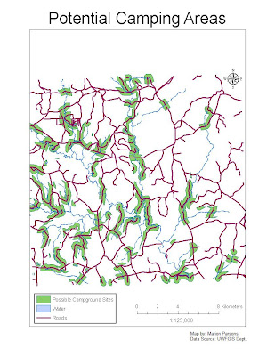
Q1: I used the Intersect Tool on the second trial of the exercise. I had the results of both methods on the map, and compared them by turning one or the other off and on several times. I could not find any differences. The Intersect Tool was what I had expected to use as I worked the problem the first time. Using the Union Tool was a good demostration of the princilple that there are always several ways to reach the same result.

Q2: I used the Erase Tool to eliminate the parts of the selected areas that overlaped the conservation areas. That seemed to be the most efficient way to remove sections that needed to be excluded in the final analysis.

Q3: There were 72 features in the final layer. The largest has an area of 7,765,034 square meters, and the smallest is 748 square meters.

Flashback to Data Search

My primary problem with this section of the lab assignment was re-projecting one DOQQ. All four came from the same source, and I thought were in the same projection. But there is apparently a critical difference between GCS_North_American_1983 and GCS_North_American_1983_CSRS. I didn’t notice the minor difference at first, until the latter could not be re-projected. ArcCatalog closed abruptly each time I tried to perform the operation. I eventually downloaded other DOQQ files and had no problem.
I added the USGS Quad background, which I clipped to the county boundary. I did not have to clip my other layers (I was able to download already clipped layers for my county), and wanted to practice that part of the lab.
I was eventually able to research CSRS, and discovered it is the Canadian Spatial Reference System, which is a 3-dimentional system. It includes data not only on height (elevation?) but gravity and earth rotation. It’s no wonder ArcCatalog choked on it.
I don’t know why one of a set of four DOQQ files was in that format, unless LABINS is in the process of converting to that format.

Module 7: Data Editing

Projection: Florida State Plane North

I have actually done this type of editing before. I used to create a lot of vector maps my office needed from georeferenced aerial photos. I did learn a few new methods and updates to the software. My biggest problem is being too perfectionist in following the roads and building outlines. I tend to use many more vertices than are needed at the scale the map will be used.

Compared to the previous lab, this one was fun! I have always been intersted in georeferencing aerial photos, but never had the access to a version of ArcGIS that included that capabiity. I did have to delete several control points and restart when I connected the points backward or not accurately enough.

Data Scavenger Hunt

I actually got rather carried away looking at all the possible data sets. Fortunately, almost all that I ended up using were in the Albers Equal Area projection, and I had to do very little re-projecting. I selected out the major roads fron a file that seemed to have every dirt trail in the marshes, cattle ranches and citrus groves. I removed 'swamps/marshes' fronm the hydrology layers leaving only streams, rivers, ponds and lakes - most of this county seems to be wetlands.

I wanted to use the Invasive Plants data with the Strategic Habitat Conservation Areas, but there was only one point in Okeechobee County in a state -wide data set. I think the conservation and wetlands combination makes a logical pair.

I will post the raster data late(r). I have only 4 hours before I have to get up for work.

The Earthquake in Haiti

This layer package was on the ESRI web site for resources on the Haiti earthquake. The base layer is an aerial photo, and the overlay is from the USGS sensors that measured the strength of the tremors at several distances from the epicenter. This will provide an excellent indication of how much damage to expect in different areas, and what locations may be sfe to relocate the population.

A Tale of Three Projections

The task this week was to take one shapefile and re-project it from the original to two other systems, then calculate the area of four counties.

It was emphasized in the reading assignment that there are errors associated with all projections, due to the difficulty of transforming an 'oblate elipsoid' onto a flat surface. It was not surprising that the calculated ares of the four counties varied. Each projection has a different base reference point, and the farther from that point, the greater the distortion.